
Early characterizations of the mid-latitude, dayside hydromagnetic response to upstream solar wind conditions: 1980
space-weather time-series data-science statistics The solar wind speeds up. It slows down. It blows by Earth at a breath-taking million miles per mile on a lethargic day. Double that when it’s feeling frisky.
As the quasi-stable electrical current systems and plasma regions in the Sun’s corona slowly vary, associated low-frequency magnetic disturbances propagate out into the solar system, not at the speed of light in vacuum (as for example disturbances in the optical band might do), but more-or-less in sync with the flow of the extremely conductive solar wind plasma. This solar wind-associated magnetic field is often called the interplanetary magnetic field [IMF].
Circa 1980, when Allan Wolfe wrote the two papers I am discussing today (see Wolfe1980a and Wolfe1980b below), space scientists were trying to establish what connections, if any, existed between interplanetary parameters upstream in the solar wind and hydromagnetic [HM] energy measured by magnetometers on the ground (a “hydromagnetic wave” is the cooler, old school term for what is more often today referred to as a “magnetohydrodynamic wave”). The solar wind speed (“velocity effect”) and the direction of the IMF (“angle effect”) were theoretically justified as major factors in controlling the hydromagnetic energy levels at Earth’s surface. In order to verify or nullify these hypotheses, the task was to get a spacecraft just ahead of the Earth in the solar wind so observational researchers could analyze the data obtained in this region with data obtained on the ground.
The Velocity Effect
The idea goes like this: increases in the solar wind speed just upstream of Earth’s bow shock induce faster plasma flows earthward of the bow shock in the magnetosheath [Dryer1966, Spreiter1966]. The magnetosheath plasma flows antisunward, continuously grazing by Earth’s magnetopause. Increases the speed of the magnetosheath plasma relative to the magnetopause are associated with increased probability of inducing a Kelvin-Helmholtz instability [KHI] at the magnetopause [Atkinson1966, Southwood1974], which is associated with the generation of hydromagnetic waves inside the magnetosphere. The generated HM waves, in turn, often excite field line resonances [FLRs], ultimately enhancing the hydromagnetic activity at ground level [Radoski1966, Chen1974, Southwood1974].
The Angle Effect
The bow shock is—you guessed it—a type of shock. It is upstream of Earth’s magnetosphere in the solar wind (“sunward of the magnetosphere”). Hydromagnetic waves are generated at this shock and, as the hypothesis goes [Greenstadt1973], these waves are more readily transported to Earth’s magnetopause when the IMF is predominately lying in the ecliptic plane—that is, when the IMF has little-to-no north or south component. To measure this, we use the “cone angle” of the IMF, defined as
\[acos(|Bx|/B)\]where Bx is the magnetic field component along the sunward/antisunward axis. The idea is that if the waves are more readily transported to the magnetopause, then if they can transmit through the magnetopause [Fejer1963, Wolfe1975], they can in turn excite FLRs inside the magnetosphere and cause variations in the hydromagnetic energy levels measured on the ground [Radoski1966, Chen1974, Southwood1974].
The Work of Wolfe
Study #1:
In an attempt to test the “velocity effect” and “angle effect” hypotheses, in Wolfe1980a, the authors use recently obtained upstream solar wind data obtained by the spacecraft IMP J (also known as Imp 8) to compare with dayside ground-based magnetometer time series data (defined as any of the 1-hour integer-to-integer intervals between 0600-1800 local time) recorded at a mid-latitude site (located in New Hampshire) during two time periods when IMP J was upstream of the bow shock.
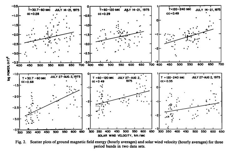
During the first interval, the authors show that for three hydromagnetic frequency bands (periodicity bands of 30.7-60, 60-120, and 120-240 seconds, which are proxies for the more traditionally defined Pc3 [10-45 s], Pc4 [45-150 s], and Pc5 [150-600] bands), the solar wind speed appears to be the dominant independent variable. However, he goes on to show that during this time interval, the IMF cone angle is correlated with the solar wind speed. Therefore, by employing a regression analysis, any detectable relationship between the solar wind speed or the IMF cone angle with the mid-latitude ground-level HM energy is confounded—that is, if and when these two upstream solar wind variables are correlated, it isn’t clear if the detected relationships with ground-level HM energy are exclusively due to the velocity effect, the angle effect, or both the velocity and the angle effect.
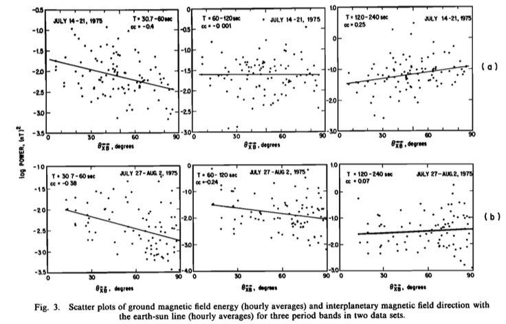
To address this, Wolfe shows that during the second interval of study there is no such correlation between the IMF direction and solar wind speed, and so the two variables can be regarded as independent. In these circumstances, he is again able to present a strong case in favor of the velocity effect. However, the case for the angle effect is more subtle: Wolfe finds that there is a frequency dependence associated with the angle effect. The analysis shows that only the highest frequency band (the “proxy Pc3” band) has energy strongly controlled by the IMF cone angle. Wolfe is unable to explain this beyond speculation (e.g., natural band-pass filtering at the shock).
Study #2
In Wolfe1980b, the dayside ground-based magnetometer data set at mid-latitude site in New Hampshire is expanded to cover four time intervals when IMP J is beyond the bow shock in the upstream solar wind. The data is collated into one large-by-the-day’s-standards data set to mine significant overall relationships from.
In this study, Wolfe wants to further quantify relative importance of the velocity and angle effects in controlling the ground-level dayside hydromagnetic energy at mid-latitudes, but also wants to know if these effects are possibly due to other underlying parameters in the solar wind. To address this, Wolfe scouts out confounding variables—that is, to uncover solar wind variables that are not independent of each other—by looking at scatter plots and computing the correlations between 8 solar wind parameters:
- Bulk Speed: \(V_{SW}\)
- Cone Angle: \(\theta_{xB}\)
- Magnetic Field Components \(B_{X}, B_{Y}, B_{Z}\)
- Magetic Field Strength: \(B_{}\)
- Proton Number Density: \(N_{p}\)
- Proton Temperature: \(T_{p}\)
Wolfe shows an extremely strong correlation between temperature and speed, no correlation between speed and cone angle, and a strong nonlinear relationship between speed and density. These results prompt the question: Is it possible that the velocity effect is in fact not an effect of velocity, but instead due to solar wind temperature or density? Looking at the scatterplot and correlation coefficient of solar wind temperature versus ground-level HM energy, one would be very inclined to posit a causal relationship.
To identify and quantify the solar wind parameters important in controlling ground-level hydromagnetic energy, Wolfe implements a sequence of multiple linear regression [MLR] analyses (stepwise MLR) on the 8 solar wind parameters. To indicate the importance of each variable in a given MLR, the T Ratio is used (aka, t-statistic)—that is, the ratio between the coefficients (slopes) of each (presumably) independent variable and their associated errors. The larger the T Ratios, the more important Wolfe considers the variable in the fit.
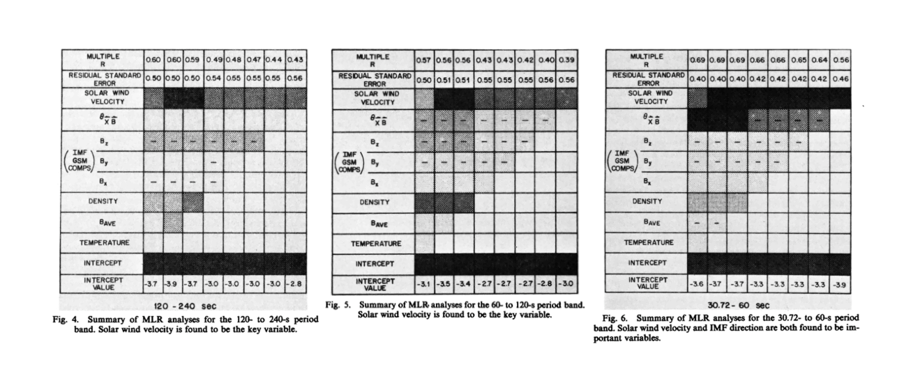
This type of analysis allows Wolfe to show justification that the velocity effect is very likely due to velocity—not temperature or density. The high correlation found between the solar wind temperature and the ground-level HM energy—judging by T Ratios and various sequences of stepwise MLR—is likely due to the high correlation between the temperature and speed. The importance of solar wind density is not ruled out: for most of the MLR analyses, its inclusion causes a sharp reduction in residual error and steep rise in the correlation. However, its predictive power pales in comparison to solar wind speed, and given the relationship it was shown to have with speed, at least some of its predictive power is likely due to speed. Therefore, in the current study, Wolfe looks no further into the “density effect.”
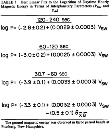
Ultimately, the study further demonstrates and justifies the velocity and angle effects, concluding that they are indeed the dominant solar parameters controlling HM energy levels on the ground, noting the possible importance of density. The study more clearly shows that the angle effect has a frequency dependence, but adds no explanation beyond further speculations as to the cause. It concludes with equations between the solar wind speed, cone angle, and ground-level HM energy for the three inspected frequency bands, which can be used in either direction — as ground-based solar wind probes or space-based estimates of mid-latitude ground measurements on the dayside!
Limitations of the Study
Having noted what Wolfe’s studies established, it is just as important to note what Wolfe did not establish or look at in these two studies. The list below is in no way a criticism of these two papers—in fact, much of what is listed below was carried out by Wolfe and his contemporaries in the years soon after (or, if not, the decades thereafter!). This section serves to demonstrate ways in which an observational science moves forward.
(1) Polarization
Wolfe only analyses the effect that the solar wind parameters have on the magnetic north component. Being a vectorial quantity, there are two further components that one can look at—the magnetic east and vertical components.
(2) Latitude dependence of the MLR analyses: These studies looked at a single mid-latitude magnetometer to characterize the mid-latitude dayside hydromagnetic response to upstream solar wind parameters. One might be interested in comparing the MLR analyses of multiple mid-latitude magnetometers in some span (e.g., 30-55* magnetic latitude). Are the dependencies on solar wind speed and cone angle the same in this mid-latitude interval? If not, then why not? For example, this could shed light on the perplexing frequency dependence of ground-level hydromagnetic energy on cone angle, which was not understood in this study.
(3) Local time dependence: As of 2015, we have access to years of upstream solar wind data thanks to missions like ACE and Wind. But at the time of these two studies, Wolfe had to find time periods in which IMP J was beyond the bow shock, and so had a limited collection of several-day spans of upstream solar wind data. Although Wolfe was aware that a local time MLR analysis would have been ideal (e.g., 1-hour bins between 0600 and 1800 local time), having only 336 1-hour dayside bins means that, e.g., for 1-hour local time bins, there would only be 28 solar wind data points to compare to for each bin. (Note: in a follow-up paper, Wolfe and co-authors actually do just this, noting that it is enough data since for each time bin there is ~24 hours between data points and little-to-no risk of autocorrelation or repeat measurements affecting the confidence levels.)
(4) Seasonal Dependence
Note that in both papers, the data intervals only cover summertime dates. One might further ask if the established relationships vary by season—summer, winter, and the equinoxes.
(5) Hemispheric Asymmetries
Since southern winter occurs during northern summer, this is similar to investigating the seasonal dependencies of the relationships found between the upstream solar wind parameters and the ground-level HM energy. However, it is still viable to ask if even the seasonal dependencies vary by hemisphere.
(6) Time resolution: Wolfe primarily looked at 1-hour time bins, checking his results afterwards with 6-hour time bins to test against distortions of the statistical significant due to autocorrelations in the 1-hour time steps. Looking at higher time resolutions was not considered due to autocorrelation considerations, which can be dealt with, but was slight overkill for the current studies. Better time resolution, for example (as Wolfe noted), could help understand the frequency dependence of the hydromagnetic spectra on cone angle since cone angle can change many times over in a given hour.
(7) Space weather dependence: that is, how do the observed relationships change when looking at times when corotating interaction regions [CIRs] are brushing by the Earth versus coronal mass ejections versus “uneventful” solar wind conditions? Again, due to the lack of solar wind data circa 1980, this was not likely a question that could be reasonably be answered. Also, given that researchers were still establishing basic connections, this type of breakdown-by-event-type would have been like putting on your shoes before your socks.
(8) Nightside dependence: the nightside is an obvious “next study” since Wolfe’s two 1980 papers only covered the dayside. Even if one suspected that nightside activity was not directly driven by upstream solar wind conditions, it is important to check and see.
(9) Other solar wind parameters: Wolfe looked at a bunch, but one could always look at more, e.g., the ratio of helium ions to hydrogen or the clock angle.
(10) Ionospheric parameters: The ionosphere acts at a filter between the happenings in the magnetosphere and the activity observed on the ground, so it is straightforward that changes in the ionosphere (electron density, conductance, etc) serve to represent different filters acting on an incoming signal. However, if a small data set is the problem, such a study represents possibly unreasonable constraints given that the researcher is now also required to restrict the study to times when a satellite was overhead and able to record such ionospheric parameters.
(11) Additional hydromagnetic frequency bands: Wolfe and his colleagues looked at what I call proxy Pc bands: a proxy Pc3 band, a proxy Pc4 band, and a proxy for the high-frequency end of the Pc5 band. Looking at the full Pc5 band, and even the Pc6 band, would be nice, although using a short-time Fourier transform technique might be too restrictive in that the longer window that is necessary for the Pc5 and Pc6 bands might not localize the dynamics of the Pc3 band well. A multi-resolution wavelet analysis could be performed to overcome this.
More on Wolfe’s Data Analysis
I first wrote this incorporating the analysis aspects into the main narrative, but this impeded the flow of physical ideas with technical jargon from statistics and time series analysis. I figured I would save it for the end for more ambitious readers.
The Logarithm Of Energy
Note that all regressions employ the logarithm of energy as the dependent variable. The actual relationships between the solar wind and the mid-latitude, ground-level HM energy are nonlinear.
Estimating Ground-Level HM Energy
In both studies, to estimate the dayside hydromagnetic energy on the ground, Wolfe first splits up the data set into 1-hour segments, discarding any of the segments on the nightside (1800-0600). Each of the remaining data segments are equally considered “dayside” segments, not explicitly differentiating effects that might be dependent on local time. For each dayside segment in his data set, he then computes the power spectral density of the magnetic north component (ignoring the magnetic east and vertical components during these early studies) by tapering each segment with a Thomson window and applying an FFT [Thomson1976]; this provides estimates of the HM energy density [nT^2/Hz]. Since Wolfe is interested in how the upstream solar wind controls energy contained in distinct frequency bands, he defines three bands of interest and band-integrates the spectral density. Note that while this provides a measure of energy in these bands, it ignores if the energy is due to an incoherent “power law” spectrum of geomagnetic noise (colored noise), or if any coherent waves are present (significant bumps above the background noise).
Computing Hourly Averages of Cone Angle
| The cone angle is defined as (\theta_{xB}=arccos( | B_{X} | /B)). The IMP J magnetic field data has a temporal resolution of about 15.36 seconds. However, Wolfe downsamples the original time series (aka decimation) of each magnetic field component into a new time series with 1-hour temporal resolution—of which the simplest way is to take averages of consecutive, independent 1-hour time bins. The cone angle itself is not downsampled itself; the “hourly average” of the cone angle is defined in terms of the decimated magnetic field components. |
Hedging Against Autocorrelation
In both studies, to further establish the results, Wolfe downsamples each of the data sets to 6-hour temporal resolution and performs further regression analyses. He does this to hedge against false confidence in the significance of his results due to autocorrelations present in the 1-hour resolution data. The additional analyses provide further justification of the initial findings. In the second paper [Wolfe1980b], both the 1-hour and 6-hour time resolved data sets have enough data points to establish correlations with significances at the 99.9% level, assuming no autocorrelation. (For more on the effect of autocorrelation on estimates of correlation and its significance in a geophysical setting, see Carter1977.)
Stepwise Multiple Linear Regression
The recipe goes like this:
1. Choose a sequence of presumably independent parameters (they need not actually be independent, but at the beginning of the analysis we pretend they are).
2. Perform MLR and note the correlation coefficient, the residual standard error, and the coefficient and error of each supposedly independent parameter.
3. Remove the last variable from the sequence chosen in (1).
4. Repeat (2) and (3) until there is only one variable left.
5. Repeat (1)-(4) on additional permutations of the parameter set.
Main References
| Wolfe1980a: A. Wolfe, L. J. Lanzerotti, and C. G. Maclennan: Dependence of Hydromagnetic Energy Spectra on Solar Wind Velocity and Interplanetary Magnetic Field Direction |
|
Wolfe1980b: A. Wolfe: Dependence of Mid-Latitude Hydromagnetic Energy Spectra on Solar Wind Velocity and Interplanetary Magnetic Field Direction |
Other References