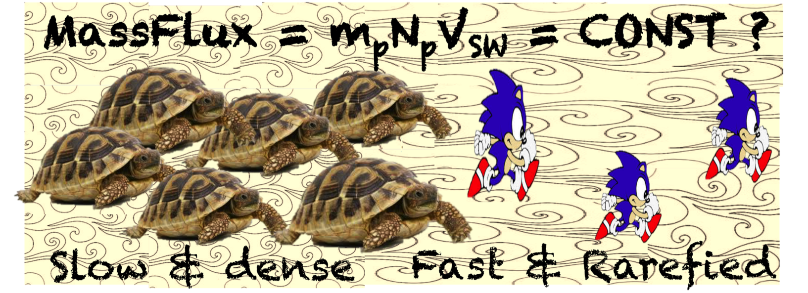
In a meta-analysis of early (1980-82) papers by Allan Wolfe (and Co) on the upstream solar wind control of ground-level hydromagnetic [GLHM] activity (a.k.a. ULF waves), I conjectured that the data analysis in Wolfe1980b indicates that the mass flux of the solar wind might be constant. Wolfe showed that there was a strong relationship between the upstream solar wind speed and density, the scatterplot illustrating that the upstream density to decay nonlinearly as a function of the speed. It occurred to me that the scatterplot of \(V_{SW}\) vs \(N_{p}\) looked fairly hyperbolic, as if \(N_{p}=\frac{A}{V_{SW}}\)

This conjecture had implications for Wolfe’s conclusions and analyses in his other papers:

1. Given the solar wind speed is considered a primary driver of GLHM energy in the context of correlation (a measure of linearly co-varying observables), then it should be expected that the density would appear to be an unimportant upstream parameter since its covariation with GLHM energy would be hyperbolic.
2. If the mass flux (\(\mathscr{M}=m_{p}N_{p}V_{SW}\)) is constant, this means that the momentum flux (\(\mathscr{P}=m_{p}N_{p}V_{SW}^{2}\)) is really a measure of \(V_{SW}\) (i.e., \(\mathscr{P}=BV_{SW}\)) and the kinetic energy flux density (\(f_{k}=\frac{1}{2}m_{p}N_{p}V_{SW}^{3}\)) is really a measure of \(V_{SW}^{2}\) (\(f_{k}=CV_{SW}^{2}\)), indicating that a polynomial regression on solar wind speed alone might suffice for Wolfe’s purposes:

log(GLHM Energy) = \(A+BV+CV^{2}+DV^{3}\)

As I thought about the constancy of the mass flux in the solar wind since these posts, I realized that I hadn’t come up with this idea independently—even if, at the moment, it had felt like that. I had heard about it before, while attending the Heliophysics Summer School, in a session led by Justin Kasper (pdf). In the magnetospheric community, the solar wind is an input: in a sense, we can take it empirically at face value. But in the solar physics community, the solar wind is an output—and so understanding why the solar wind’s mass flux at the distance of Earth’s orbit is approximately constant is actually a huge issue (e.g., 1989: Withbroe: The Solar Wind Mass Flux). I’m not even sure if it is resolved at the moment. But I digress!

While continuing my readings of Wolfe’s work throughout the 1980s, I wondered if the constancy of the solar wind mass flux (given that it is indeed constant) might be an important, but largely unconsidered, feature in his ongoing analyses and interpretations… So I began playing with some solar wind data from the Advanced Composition Explorer [ACE]. To my surprise, while looking at about 2-3 months of solar wind speed and density data data (64-sec temporal resolution), I could not prove to myself that the mass flux was constant. Not even after separating it into slow, moderate, and fast categories.

This weirded me out… So I started Googling and Google-Scholaring.

I found that in the older papers that mention “constant mass flux” in the solar wind, they are referring to the broad strokes, e.g., Burlaga and Ogilvie [1973] looked at median quantities over entire solar rotation periods when they uncovered this relationship.

The minute-to-minute fluctuations in the solar wind speed and density over the course of three months does not depict a constant solar wind mass flux because the mass flux is simply not a constant at this time scale. However, it might be approximately so on an hourly time scale given that Wolfe’s analyses used hourly averages of solar wind parameters.

The leap from the median speed and density over a solar rotation (~27-28 days) to the hourly time scale is quite large, so I decided to look at daily median quantities over the whole year of 2001. 

On the daily timescale, the scatterplots indeed start to look hyperbolic, as if the upstream solar wind density is inversely proportional to the speed like \(N_{p} = \frac{A}{V_{SW}}\). If this relationship is true, then would should expect a fairly linear relationship between \(V_{SW}\) and \(1/N_{p}\) since this would be equivalent to correlating \(V_{SW}\) and \(\frac{1}{A}V_{SW}\).

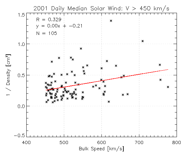
Indeed, you get a pretty straight line. The correlation increases if you scatterplot only on fast solar wind: \(N_{p}[V_{SW} > 450 \quad km/s]\) vs \(V_{SW}[V_{SW} > 450 \quad km/s]\). However, although there is a relationship, the solar wind speed only explains ~10% of the variance in the inverse density.

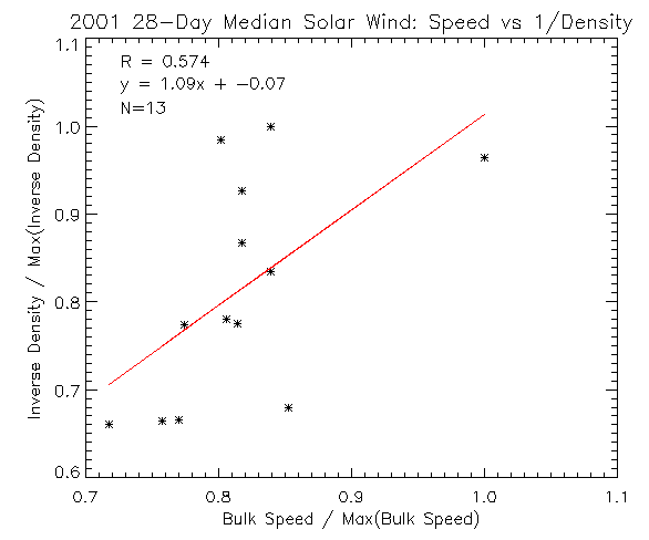
Using 28-day medians, the N=A/V relationship becomes much stronger. The correlation coefficient suggests that ~33% of the variance in the inverse density is explained by the solar wind speed. However, it is only 13 data points in the single-year of 2001, so this gives us a rather large standard error on the correlation coefficient:

\[SE_{corr}=\frac{\sqrt(1-R^{2})}{\sqrt(N-2)}\sim=0.25\]

It would take further analysis to establish the details of the relationship between solar wind speed and density, e.g., a multi-year study of solar wind properties over many solar rotations. However, given just a little bit of data analysis, we were able to answer our question: Is the solar wind mass flux at Earth constant, variable, or both?

The answer, of course, is both: it depends on what time scale you’re interested in (minutes, hours, days, or solar rotation periods) and how much variation is encapsulated in one’s definition of constant (e.g., the temperature in a room might be continuously fluctuating within a tenth of a degree about 68 degrees, but most of us wouldn’t consider the temperature in the room “constant”).