The Angle Between Two Data Sets

[ statistics ]

Did you know that a correlation is similar to an inner product between two data sets?

“Huh? Never heard of it.”

Oh Reader! I’m sure you’re kidding. But just in case: an inner product is a measure that allows one to quantify how similar two mathematical objects are. If we’re talking about two criss-crossing lines in 3D Euclidean space, this amounts to measuring if they are collinear, perpendicular, or somewhere in between. This means that an inner product allows at least a qualitative measure of the “angle” between two mathematical objects. Any old inner product can, at the least, tell us whether or not two objects are “perpendicular” or not. If one uses a normalized inner product, then one can fully measure the angles between objects.

There might be a lot of terminology here, so an example will help.

A typical inner product in the normal Euclidean setting in 2D or 3D space is the dot product. Say you have two 3D vectors, $A = (A_{1},A_{2},A_{3})$ and $B=(B_{1},B_{2},B_{3})$. (The results below are applicable to 2D vectors by simply assuming that $A_{3}=0$ and $B_{3}=0$.) The dot product of these two vectors can be written in two important ways, both of which will give you the same answer. Deciding on which identity you use simply depends on your preference, or possibly how you collected your data: did you measure rectilinear components, magnitudes and angles, or both?

Inner Product (Def1): $\quad Dot(A,B) = \Sigma_{i=1}^{3}A_{i}B_{i} = A_{1}B_{1}+A_{2}B_{2}+A_{3}B_{3}$
Inner Product (Def2): $\quad\quad Dot(A,B) = \|A\|\|B\|cos(\theta)$

Here we use the notation $\|A\|$ to denote the norm (aka the length) of the vector A. The norm is defined as follows:

IP-Induced Norm: $\quad\quad Norm(A) = \sqrt{Dot(A,A)} = \sqrt{\|A\|^{2}cos(0)} = \|A\|$

An important observation here is that the inner product (qualitative mixed measurement of angles and lengths) on the space naturally induces a definition of the norm (length) on that space.

Furthermore, the equality in Eq(2) tells us that if we can define a normalized inner product rather easily:

Normalized Inner Product: $\quad\quad NormDot(A,B) = \frac{Dot(A,B)}{\|A\|\|B\|} = cos(\theta)$

Having this normalized inner product, we then see that we can quantitatively compute the angle between any two vectors in this space:

Angle: $\quad\quad \theta =acos\left(\frac{A\cdot B}{\|A\|\|B\|}\right)$

The important take-away here is that in these simple vector spaces, the notions of vector components, vector magnitudes, and angles between vectors are all intuitive. In fact, mathematically speaking, the generalized definitions of inner product and norm was motivated by the desire to generalize these geometric notions to other mathematical spaces.

The ideas generalize to N-dimensional Euclidean spaces without any required thinking: all of the definitions we worked out above are immediately applicable to N-dimensional vectors. That is, although we might not be able to picture it in our mind, in a real-valued N-dimensional space, we mathematically have the quantified notions of vector magnitude, vector components, and the angle between two vectors. If we’re interested in variables that are composed of complex numbers, these definitions even generalize to complex vector spaces with very little thought (for example, the N-dimensional Hilbert spaces in quantum mechanics). Most things we measure on a day-to-day basis, however, have real-number values (stock prices, wind speed, heights, weights, etc), so for the moment, let’s not make the situation any more complex.

“Pun intended?”

Damn right, Reader. Pun intended!

From N-Dimensional Euclidean Space to N-Element Data Sets

We’ll get from Euclidean Space to Data Space by imagining that we’ve collected two associated sets of mean-subtracted numerical data, $A = (A_{1},A_{2},...,A_{N})$ and $B = (B_{1},B_{2},...,B_{N})$. The “association” aspect is important because correlation can only be used to measure a relationship between two stochastic/random variables whose instances can be meaningfully paired together: for two time series, the association might be the instants of time each data stream were simultaneously measured at; if it a data set about people (e.g., height, weight, income), then the association tying the two data sets together are the individuals. If you cannot meaningfully pair two data sets, then you cannot compute a correlation, e.g., if you have an N-element data set of rock sizes and another N-elements data set of people’s heights, how would you meaningfully pair these data sets? The answer is that you can’t—not unless you’re doing a study that specifically pairs these variables, e.g., if you’ve collected data concerning what-sized rock different individuals first pick up when they are placed in a rock quarry for an hour.

The Geometry of Statistics

In the statistical setting, the sample covariance for a mean-subtracted data set is written:

\[\quad\quad Cov(A,B) = \frac{1}{N-1}\Sigma_{i}^{N}Α_{i}B_{i}\]

The sample standard deviation is just the square root of the sample variance—and variance is just a special case of covariance:

\[std(A) = \sqrt{Var(A)} = \sqrt{Cov(A,A)} = \frac{1}{N-1}\Sigma_{i=1}^{N}A_{i}^{2}\]

The sampled correlation coefficient has the following definition:

\[\rho(A,B) = \frac{Cov(A,B)}{\sqrt{Var(A)Var(B)}}\]

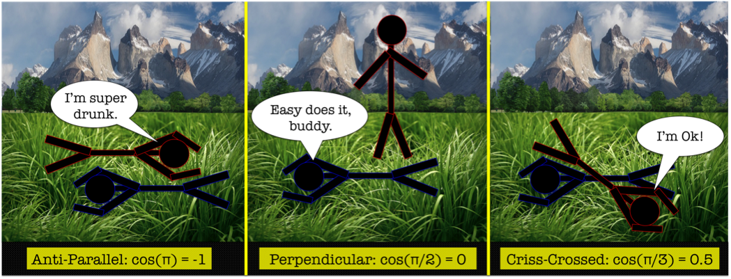
Note that you can explicitly compute an “angle between data sets” by allowing the above equation to generalize to this situation:

\[Cov(A,B) = std(A)StdDev(B)cos(\theta)\]
\[\theta = acos\left(\frac{Cov(A,B)}{std(A)std(B)}\right)\]

Given this generalization to the statistical setting, you can see that the correlation coefficient is not just similar to a cosine, but is literally a cosine:

$$\rho(A,B) = \frac{Cov(A,B)}{std(A)std(B)} = cos(\theta)$$

The above equations are marked as asterisked versions of the previous equations for a pretty obvious reason. C

ovariance looks suggestive of an inner product, doesn’t it? An inner product on a real-valued vector space is characterized by linearity (IP(aX+Z,Y)=aIP(X,Y)+IP(Z,Y), symmetry in its arguments (IP(A,B)=IP(B,A)), and positive-definiteness (IP(X,Y) (\ge) 0, the equality of which is reached only for X=Y=0).

Correlation is certainly symmetric in its arguments and positive definite. Without further thought, it even satisfies the scalar portion of the linearity property (IP(aX,Y)=aIP(X,Y)). If we can conjure up a useful or believable definition of vector addition (which seems possible), then correlation is an inner product! By analogy to Euclidean space, then, a covariance is some mixed measure of magnitude and angle between two mean-subtracted data sets. Just like the Euclidean case, this particular inner product induces a norm—the standard deviation—which is somehow, by analogy, a measure of the data vector’s magnitude. We can also now see that the correlation coefficient is a normalized inner product:—a measure of the angle between two data vectors.

I think maybe the craziest thing here is that the statistical concepts we’re so familiar with in the data setting are not just analogous to geometrical notions from Euclidean space, but literally are the geometrical notions fudged by a scalar—at least for mean-subtracted data sets.

Implications

Correlations coefficients are not additive quantities, and the geometric notions presented here should give you an idea of why. Cosines, in general, are not additive: cos(θ) + cos(φ) does not equal cos(θ+φ). However, one can find examples on the internet of people improperly computing arithmetic averages of correlation coefficients, for example, in an attempt at a meta-analysis of published results in some research field. Perhaps they think they are measuring the central tendency of the correlation coefficients, convinced that they have uncovered the true population parameter. Unfortunately, in cases like this, the arithmetic average does not necessarily represent an obvious or meaningful measure—it is not a robust measure of central tendency.

SUMMARY TABLE

	N-Dimensional Euclidean Vectors	N-Element Mean-Subtracted Data Sets	Relationship
Inner Product (Def1)	$Dot(A,B) = \Sigma_{i=1}^{N}A_{i}B_{i}$	$Cov(A,B) = \frac{1}{N-1}\Sigma_{i}^{N}Α_{i}B_{i}$	$Cov(A,B) = \frac{1}{N-1}Dot(A,B)$
Inner Product (Def2)	$Dot(A,B) = \|A\|\|B\|cos(\theta)$	$Cov(A,B) = std(A)std(B)cos(\theta)$	$Cov(A,B) = \frac{1}{N-1}Dot(A,B)$
Norm	$\|A\| = \sqrt{Dot(A,A)} $	$std(A) = \sqrt{Cov(A,A)}$	$std(A) = \sqrt{\frac{1}{N-1}}\|A\|$
Normalized Inner Product (Def1)	$NormDot(A,B) = \frac{Dot(A,B)}{\|A\|\|B\|}$	$\rho(A,B) = \frac{Cov(A,B)}{std(A)std(B)}$	$\rho(A,B) = NormDot(A,B) $
Normalized Inner Product (Def2)	$NormDot(A,B) = cos(\theta)$	$\rho(A,B) = cos(\theta)$	$\rho(A,B) = NormDot(A,B) $
Angle	$\theta = acos\left(\frac{A\cdot B}{\|A\|\|B\|}\right)$	$\theta = acos\left(\frac{Cov(A,B)}{std(A)std(B)}\right)$	$\theta=\theta$

	N-Dimensional Euclidean Vectors	N-Element Mean-Subtracted Data Sets	Relationship
Inner Product (Def1)	\(Dot(A,B) = \Sigma_{i=1}^{N}A_{i}B_{i}\)	\(Cov(A,B) = \frac{1}{N-1}\Sigma_{i}^{N}Α_{i}B_{i}\)	\(Cov(A,B) = \frac{1}{N-1}Dot(A,B)\)
Inner Product (Def2)	\(Dot(A,B) = \|A\|\|B\|cos(\theta)\)	\(Cov(A,B) = std(A)std(B)cos(\theta)\)	\(Cov(A,B) = \frac{1}{N-1}Dot(A,B)\)
Norm	\(\|A\| = \sqrt{Dot(A,A)} \)	\(std(A) = \sqrt{Cov(A,A)}\)	\(std(A) = \sqrt{\frac{1}{N-1}}\|A\|\)
Normalized Inner Product (Def1)	\(NormDot(A,B) = \frac{Dot(A,B)}{\|A\|\|B\|}\)	\(\rho(A,B) = \frac{Cov(A,B)}{std(A)std(B)}\)	\(\rho(A,B) = NormDot(A,B) \)
Normalized Inner Product (Def2)	\(NormDot(A,B) = cos(\theta)\)	\(\rho(A,B) = cos(\theta)\)	\(\rho(A,B) = NormDot(A,B) \)
Angle	\(\theta = acos\left(\frac{A\cdot B}{\|A\|\|B\|}\right)\)	\(\theta = acos\left(\frac{Cov(A,B)}{std(A)std(B)}\right)\)	\(\theta=\theta\)